|
|
< Day Day Up > |
|
We now present a linear-time string-matching algorithm due to Knuth, Morris, and Pratt. Their algorithm avoids the computation of the transition function δ altogether, and its matching time is Θ(n) using just an auxiliary function π[1 ‥ m] precomputed from the pattern in time Θ(m). The array π allows the transition function δ to be computed efficiently (in an amortized sense) "on the fly" as needed. Roughly speaking, for any state q = 0, 1, . . . , m and any character a ∈ Σ, the value π[q] contains the information that is independent of a and is needed to compute δ(q, a). (This remark will be clarified shortly.) Since the array π has only m entries, whereas δ has Θ(m |Σ|) entries, we save a factor of |Σ| in the preprocessing time by computing π rather than δ.
The prefix function π for a pattern encapsulates knowledge about how the pattern matches against shifts of itself. This information can be used to avoid testing useless shifts in the naive pattern-matching algorithm or to avoid the precomputation of δ for a string-matching automaton.
Consider the operation of the naive string matcher. Figure 32.10(a) shows a particular shift s of a template containing the pattern P = ababaca against a text T. For this example, q = 5 of the characters have matched successfully, but the 6th pattern character fails to match the corresponding text character. The information that q characters have matched successfully determines the corresponding text characters. Knowing these q text characters allows us to determine immediately that certain shifts are invalid. In the example of the figure, the shift s + 1 is necessarily invalid, since the first pattern character (a) would be aligned with a text character that is known to match with the second pattern character (b). The shift s′ = s + 2 shown in part (b) of the figure, however, aligns the first three pattern characters with three text characters that must necessarily match. In general, it is useful to know the answer to the following question:
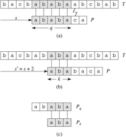
Given that pattern characters P[1 ‥ q] match text characters T[s + 1 ‥ s + q], what is the least shift s′ > s such that
where s′ + k = s + q?
Such a shift s′ is the first shift greater than s that is not necessarily invalid due to our knowledge of T[s + 1 ‥ s + q]. In the best case, we have that s′ = s + q, and shifts s + 1, s + 2, . . . , s + q - 1 are all immediately ruled out. In any case, at the new shift s′ we don't need to compare the first k characters of P with the corresponding characters of T, since we are guaranteed that they match by equation (32.5).
The necessary information can be precomputed by comparing the pattern against itself, as illustrated in Figure 32.10(c). Since T[s′ + 1 ‥ s′ + k] is part of the known portion of the text, it is a suffix of the string Pq. Equation (32.5) can therefore be interpreted as asking for the largest k < q such that Pk ⊐ Pq. Then, s′ = s+(q - k) is the next potentially valid shift. It turns out to be convenient to store the number k of matching characters at the new shift s′, rather than storing, say, s′ - s. This information can be used to speed up both the naive string-matching algorithm and the finite-automaton matcher.
We formalize the precomputation required as follows. Given a pattern P[1 ‥ m], the prefix function for the pattern P is the function π : {1, 2, . . . , m} → {0, 1, . . . , m - 1} such that
π[q] = max {k : k < q and Pk ⊐ Pq}.
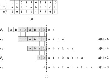
That is, π[q] is the length of the longest prefix of P that is a proper suffix of Pq. As another example, Figure 32.11(a) gives the complete prefix function π for the pattern ababababca.
The Knuth-Morris-Pratt matching algorithm is given in pseudocode below as the procedure KMP-MATCHER. It is mostly modeled after FINITE-AUTOMATON-MATCHER, as we shall see. KMP-MATCHER calls the auxiliary procedure COMPUTE-PREFIX-FUNCTION to compute π.
KMP-MATCHER(T, P)
 1 n ← length[T]
 2 m ← length[P]
 3 π ← COMPUTE-PREFIX-FUNCTION(P)
 4 q ← 0                          ▹Number of characters matched.
 5 for i ← 1 to n                 ▹Scan the text from left to right.
 6      do while q > 0 and P[q + 1] ≠ T[i]
 7             do q ← π[q]    ▹Next character does not match.
 8         if P[q + 1] = T[i]
 9            then q ← q + 1      ▹Next character matches.
10         if q = m                    ▹Is all of P matched?
11            then print "Pattern occurs with shift" i - m
12                 q ← π[q]    ▹Look for the next match.
COMPUTE-PREFIX-FUNCTION(P)
 1 m ← length[P]
 2 π[1] ← 0
 3 k ← 0
 4 for q ← 2 to m
 5      do while k > 0 and P[k + 1] ≠ P[q]
 6             do k ← π[k]
 7         if P[k + 1] = P[q]
 8            then k ← k + 1
 9         π[q] ← k
10 return π
We begin with an analysis of the running times of these procedures. Proving these procedures correct will be more complicated.
The running time of COMPUTE-PREFIX-FUNCTION is Θ(m), using the potential method of amortized analysis (see Section 17.3). We associate a potential of k with the current state k of the algorithm. This potential has an initial value of 0, by line 3. Line 6 decreases k whenever it is executed, since π[k] < k. Since π[k] ≥ 0 for all k, however, k can never become negative. The only other line that affects k is line 8, which increases k by at most one during each execution of the for loop body. Since k < q upon entering the for loop, and since q is incremented in each iteration of the for loop body, k < q always holds. (This justifies the claim that π[q] < q as well, by line 9.) We can pay for each execution of the while loop body on line 6 with the corresponding decrease in the potential function, since π[k] < k. Line 8 increases the potential function by at most one, so that the amortized cost of the loop body on lines 5-9 is O(1). Since the number of outer-loop iterations is Θ(m), and since the final potential function is at least as great as the initial potential function, the total actual worst-case running time of COMPUTE-PREFIX-FUNCTION is Θ(m).
A similar amortized analysis, using the value of q as the potential function, shows that the matching time of KMP-MATCHER is Θ(n).
Compared to FINITE-AUTOMATON-MATCHER, by using π rather than δ, we have reduced the time for preprocessing the pattern from O(m |Σ|) to Θ(m), while keeping the actual matching time bounded by Θ(n).
We start with an essential lemma showing that by iterating the prefix function π, we can enumerate all the prefixes Pk that are proper suffixes of a given prefix Pq. Let
π*[q] = {π[q], π(2)[q], π(3)[q], . . . , π(t)[q]},
where π(i)[q] is defined in terms of functional iteration, so that π(0)[q] = q and π(i+1)[q] = π[π(i)[q]] for i ≥ 1, and where it is understood that the sequence in π*[q] stops when π(t)[q] = 0 is reached. The following lemma characterizes π*[q], as Figure 32.11 illustrates.
Let P be a pattern of length m with prefix function π. Then, for q = 1, 2, . . . , m, we have π*[q] = {k : k < q and Pk ⊐ Pq}.
Proof We first prove that
If i ∈ π*[q], then i = π(u)[q] for some u > 0. We prove equation (32.6) by induction on u. For u = 1, we have i = π[q], and the claim follows since i < q and Pπ[q] ⊐ Pq. Using the relations π[i] < i and Pπ[i] ⊐ Pi and the transitivity of < and ⊐ establishes the claim for all i in π*[q]. Therefore, π*[q] ⊆ {k : k < q and Pk ⊐ Pq}.
We prove that {k : k < q and Pk ⊐ Pq} ⊆ π*[q] by contradiction. Suppose to the contrary that there is an integer in the set {k : k < q and Pk ⊐ Pq} - π*[q], and let j be the largest such value. Because π[q] is the largest value in {k : k < q and Pk ⊐ Pq} and π[q] ∈ π*[q], we must have j < π[q], and so we let j′ denote the smallest integer in π*[q] that is greater than j. (We can choose j′ = π[q] if there is no other number in π*[q] that is greater than j.) We have Pj ⊐ Pq because j ∈ {k : k < q and Pk ⊐ Pq}, and we have Pj′ ⊐ Pq because j′ ∈ π*[q]. Thus, Pj ⊐ Pj′ by Lemma 32.1, and j is the largest value less than j′ with this property. Therefore, we must have π[j′] = j and, since j′ ∈ π*[q], we must have j ∈ π*[q] as well. This contradiction proves the lemma.
The algorithm COMPUTE-PREFIX-FUNCTION computes π[q] in order for q = 1, 2, . . . , m. The computation of π[1] = 0 in line 2 of COMPUTE-PREFIX-FUNCTION is certainly correct, since π[q] < q for all q. The following lemma and its corollary will be used to prove that COMPUTE-PREFIX-FUNCTION computes π[q] correctly for q > 1.
Let P be a pattern of length m, and let π be the prefix function for P. For q = 1, 2, . . . , m, if π[q] > 0, then π[q] - 1 ∈ π*[q - 1].
Proof If r = π[q] > 0, then r < q and Pr ⊐ Pq; thus, r - 1 < q - 1 and Pr-1 ⊐ Pq-1 (by dropping the last character from Pr and Pq). By Lemma 32.5, therefore, π[q] - 1 = r - 1 ∈ π*[q - 1].
For q = 2, 3, . . . , m, define the subset Eq-1 ⊆ π*[q - 1] by
|
Eq-1 |
= |
{k ∈ π*[q - 1] : P[k + 1] = P[q]} |
|
= |
{k : k < q - 1 and Pk ⊐ Pq-1 and P[k + 1] = P[q]} (by Lemma 32.5) |
|
|
= |
{k : k < q - 1 and Pk+1 ⊐ Pq}. |
The set Eq-1 consists of the values k < q - 1 for which Pk ⊐ Pq-1 and for which Pk+1 ⊐ Pq, because P[k + 1] = P[q]. Thus, Eq-1 consists of those values k ∈ π*[q - 1] such that we can extend Pk to Pk+1 and get a proper suffix of Pq.
Let P be a pattern of length m, and let π be the prefix function for P. For q = 2, 3, . . . , m,
Proof If Eq-1 is empty, there is no k ∈ π*[q - 1] (including k = 0) for which we can extend Pk to Pk+1 and get a proper suffix of Pq. Therefore π[q] = 0.
If Eq-1 is nonempty, then for each k ∈ Eq-1 we have k + 1 < q and Pk+1 ⊐ Pq. Therefore, from the definition of π[q], we have
Note that π[q] > 0. Let r = π[q] - 1, so that r + 1 = π[q]. Since r + 1 > 0, we have P[r + 1] = P[q]. Furthermore, by Lemma 32.6, we have r ∈ π*[q - 1]. Therefore, r ∈ Eq-1, and so r ≤ max {k ∈ Eq-1} or, equivalently,
Combining equations (32.7) and (32.8) completes the proof.
We now finish the proof that COMPUTE-PREFIX-FUNCTION computes π correctly. In the procedure COMPUTE-PREFIX-FUNCTION, at the start of each iteration of the for loop of lines 4-9, we have that k = π[q - 1]. This condition is enforced by lines 2 and 3 when the loop is first entered, and it remains true in each successive iteration because of line 9. Lines 5-8 adjust k so that it now becomes the correct value of π[q]. The loop on lines 5-6 searches through all values k ∈ π*[q - 1] until one is found for which P[k + 1] = P[q]; at that point, k is the largest value in the set Eq-1, so that, by Corollary 32.7, we can set π[q] to k + 1. If no such k is found, k = 0 in line 7. If P[1] = P[q], then we should set both k and π[q] to 1; otherwise we should leave k alone and set π[q] to 0. Lines 7-9 set k and π[q] correctly in either case. This completes our proof of the correctness of COMPUTE-PREFIX-FUNCTION.
The procedure KMP-MATCHER can be viewed as a reimplementation of the procedure FINITE-AUTOMATON-MATCHER. Specifically, we shall prove that the code in lines 6-9 of KMP-MATCHER is equivalent to line 4 of FINITE-AUTOMATON-MATCHER, which sets q to δ(q, T[i]). Instead of using a stored value of δ(q, T[i]), however, this value is recomputed as necessary from p. Once we have argued that KMP-MATCHER simulates the behavior of FINITE-AUTOMATON-MATCHER, the correctness of KMP-MATCHER follows from the correctness of FINITE-AUTOMATON-MATCHER (though we shall see in a moment why line 12 in KMP-MATCHER is necessary).
The correctness of KMP-MATCHER follows from the claim that we must have either δ(q, T[i]) = 0 or δ(q, T[i]) - 1 ∈ π*[q]. To check this claim, let k = δ(q, T[i]). Then, Pk ⊐ PqT[i] by the definitions of δ and σ. Therefore, either k = 0 or else k ≥ 1 and Pk-1 ⊐ Pq by dropping the last character from both Pk and PqT[i] (in which case k - 1 ∈ π*[q]). Therefore, either k = 0 or k - 1 ∈ π*[q], proving the claim.
The claim is used as follows. Let q′ denote the value of q when line 6 is entered. We use the equivalence π*[q] = {k : k < q and Pk ⊐ Pq} from Lemma 32.5 to justify the iteration q ← π[q] that enumerates the elements of {k : Pk ⊐ Pq′}.
Lines 6-9 determine δ(q′, T[i]) by examining the elements of π*[q′] in decreasing order. The code uses the claim to begin with q = φ(Ti-1) = σ(Ti-1) and perform the iteration q ← π[q] until a q is found such that q = 0 or P[q + 1] = T[i]. In the former case, δ(q′, T[i]) = 0; in the latter case, q is the maximum element in Eq′, so that δ(q′, T[i]) = q + 1 by Corollary 32.7.
Line 12 is necessary in KMP-MATCHER to avoid a possible reference to P[m + 1] on line 6 after an occurrence of P has been found. (The argument that q = σ(Ti-1) upon the next execution of line 6 remains valid by the hint given in Exercise 32.4-6: δ(m, a) = δ(π[m], a) or, equivalently, σ(Pa) = σ(Pπ[m]a) for any a ∈ Σ.) The remaining argument for the correctness of the Knuth-Morris-Pratt algorithm follows from the correctness of FINITE-AUTOMATON-MATCHER, since we now see that KMP-MATCHER simulates the behavior of FINITE-AUTOMATON-MATCHER.
Compute the prefix function π for the pattern ababbabbabbababbabb when the alphabet is Σ = {a, b}.
Give an upper bound on the size of π*[q] as a function of q. Give an example to show that your bound is tight.
Explain how to determine the occurrences of pattern P in the text T by examining the π function for the string PT (the string of length m + n that is the concatenation of P and T).
Show how to improve KMP-MATCHER by replacing the occurrence of π in line 7 (but not line 12) by π′, where π′ is defined recursively for q = 1, 2, . . . , m by the equation
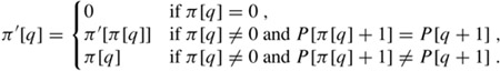
Explain why the modified algorithm is correct, and explain in what sense this modification constitutes an improvement.
Give a linear-time algorithm to determine if a text T is a cyclic rotation of another string T′. For example, arc and car are cyclic rotations of each other.
Give an efficient algorithm for computing the transition function δ for the string-matching automaton corresponding to a given pattern P. Your algorithm should run in time O(m |Σ|). (Hint: Prove that δ(q, a) = δ(π[q], a) if q = m or P[q + 1] ≠ a.)
Let yi denote the concatenation of string y with itself i times. For example, (ab)3 = ababab. We say that a string x ∈ Σ* has repetition factor r if x = yr for some string y ∈ Σ* and some r > 0. Let ρ(x) denote the largest r such that x has repetition factor r.
Give an efficient algorithm that takes as input a pattern P[1 ‥ m] and computes the value ρ(Pi) for i = 1, 2, . . . , m. What is the running time of your algorithm?
For any pattern P[1 ‥ m], let ρ*(P) be defined as max≤i≤m ρ(Pi). Prove that if the pattern P is chosen randomly from the set of all binary strings of length m, then the expected value of ρ*(P) is O(1).
Argue that the following string-matching algorithm correctly finds all occurrences of pattern P in a text T[1 ‥ n] in time O(ρ*(P)n + m).
REPETITION-MATCHER(P, T)
 1  m ← length[P]
 2  n ← length[T]
 3  k ← 1 + ρ*(P)
 4  q ← 0
 5  s ← 0
 6  while s ≤ n - m
 7      do if T[s + q + 1] = P[q + 1]
 8            then q ← q + 1
 9                 if q = m
10                    then print "Pattern occurs with shift" s
11         if q = m or T[s + q + 1] ≠ P[q + 1]
12            then s ← s + max(1, ⌈q/k⌉)
13                 q ← 0
This algorithm is due to Galil and Seiferas. By extending these ideas greatly, they obtain a linear-time string-matching algorithm that uses only O(1) storage beyond what is required for P and T.
|
|
< Day Day Up > |
|